National Reference Stations
Have a look at the file and see what is available for plotting, by downloading the file you can inspect the parameters and the Stations available.
NRSz <- planktonr::pr_get_Indices(Survey = "NRS", Type = "Zooplankton")
unique(NRSz$Parameters)
#> [1] "Biomass_mgm3"                  "AshFreeBiomass_mgm3"
#> [3] "ZoopAbundance_m3"              "CopeAbundance_m3"
#> [5] "AvgTotalLengthCopepod_mm"      "OmnivoreCarnivoreCopepodRatio"
#> [7] "NoCopepodSpecies_Sample"       "ShannonCopepodDiversity"
#> [9] "CopepodEvenness"
unique(NRSz$StationName)
#>  [1] Darwin                  Esperance               Kangaroo Island
#>  [4] Maria Island            Ningaloo                North Stradbroke Island
#>  [7] Port Hacking            Rottnest Island         Bonney Coast
#> [10] Yongala
#> 10 Levels: Darwin Yongala Ningaloo North Stradbroke Island ... Maria Island
Trend Analysis
Long term plankton monitoring can provide insights into how zooplankton abundance and biomass are changing with time. This has implications for the fish communities they support and the lower trophic levels on which they depend for energy. Abundance and biomass trends don’t necessarily show the same temporal trends, here we show zooplankton abundance by time, but biomass can also be chosen as the parameter. Seasonal cycles can also be important for understanding planktonic communities, for examples in these plots it is clear that there is a much stronger seasonal cycle at Maria Island in a temperate location than at Yongala, a more tropical station.
NRSz <- planktonr::pr_get_Indices(Survey = "NRS", Type = "Zooplankton") %>%
  filter(Parameters == "ZoopAbundance_m3") %>%
  filter(StationCode %in% c("YON", "NSI", "PHB", "MAI"))

p1 <- planktonr::pr_plot_Trends(NRSz, Trend = "Raw", method = "lm", trans = "log10")
p2 <- planktonr::pr_plot_Trends(NRSz, Trend = "Month", method = "loess")

p1 + p2 +
  ggplot2::theme(axis.title.y = ggplot2::element_blank()) + # Remove y-title from 2nd column
  plot_layout(widths = c(3, 1), guides = "collect")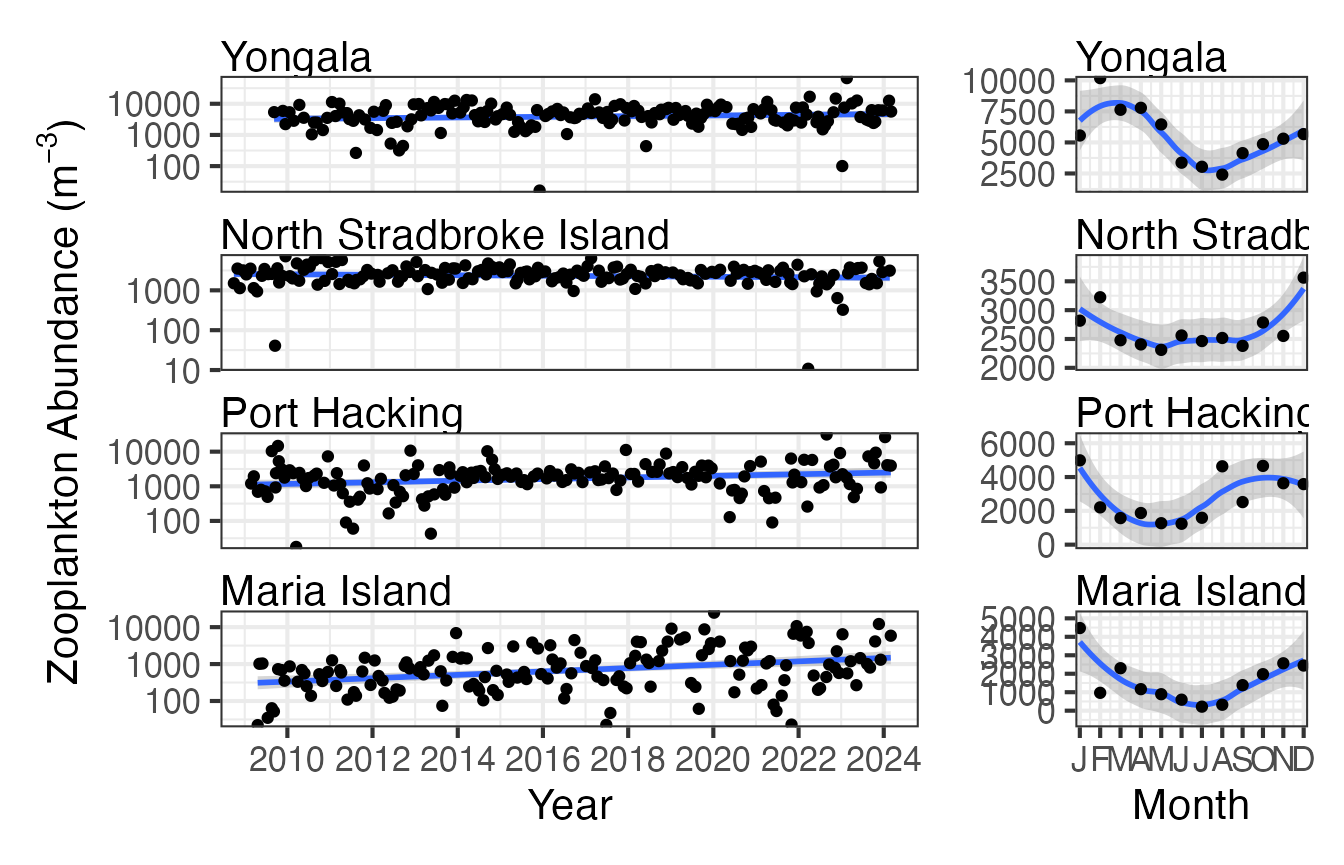
Climatologies
Here we plot the same information but change the format of the figures.
First we plot zooplankton abundance at the 4 east coast NRS stations with log10 scaling.
(p1 <- planktonr::pr_plot_TimeSeries(NRSz, trans = "log10") +
   ylab(rlang::expr(paste("Abundance (m"^-3,")"))))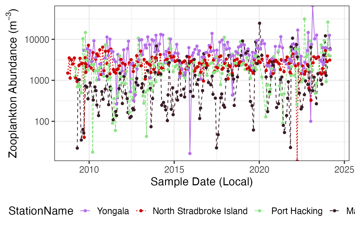
Then we can plot the same data as monthly means.
(p2 <- planktonr::pr_plot_Climatology(NRSz, Trend = "Month", trans = "log10") +
   ylab(rlang::expr(paste("Abundance (m"^-3,")"))))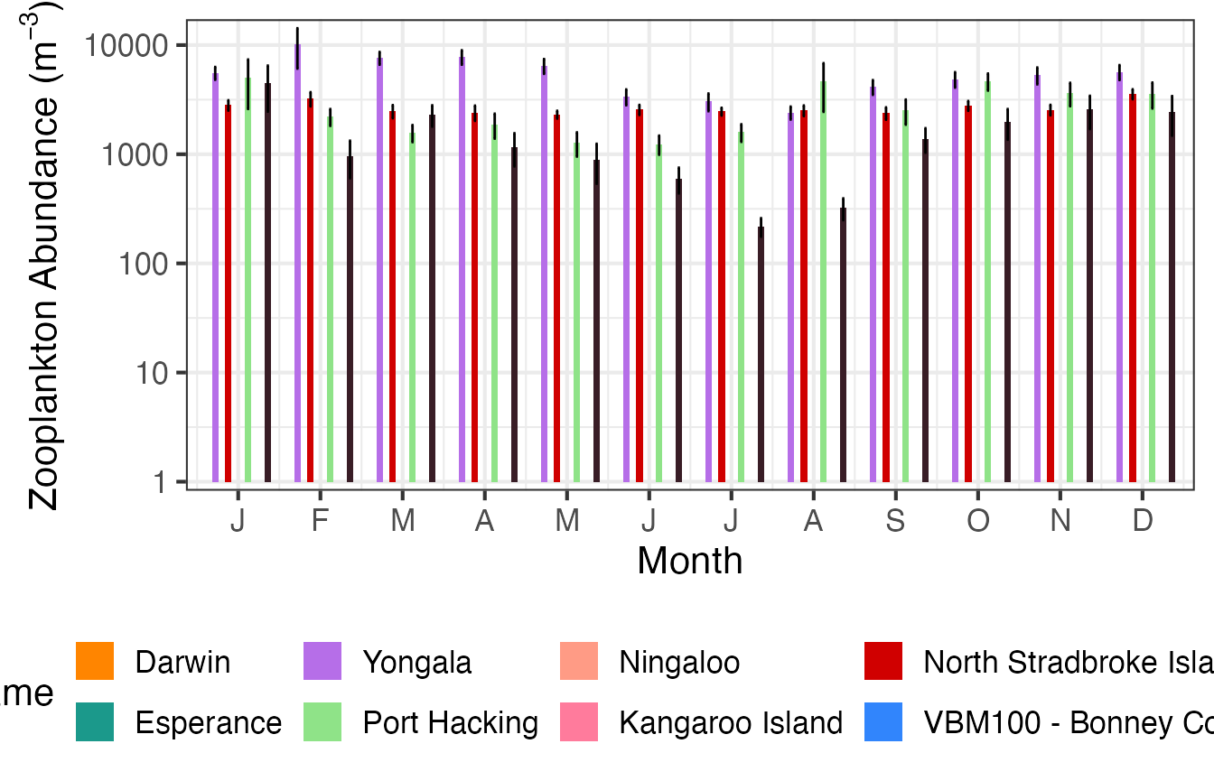
And then as Annual means.
(p3 <- planktonr::pr_plot_Climatology(NRSz, Trend = "Year", trans = "log10") +
   ylab(rlang::expr(paste("Abundance (m"^-3,")"))))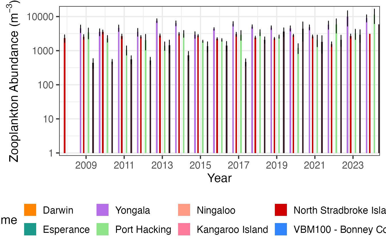
Functional Groups
We can also gain a lot of insight into the community structure by looking at how the composition (or proportions) of the functional groups changes over time, long term and seasonally. In this function we have chosen some of the more important function groups and plotted them as a time series and a seasonal cycle. Again you can see that Maria Island demonstrates a strong seasonal pattern with lower abundances in all groups during winter.
FGz <- pr_get_FuncGroups(Survey = "NRS", Type = "Zooplankton") %>%
  dplyr::filter(StationCode %in% c("ROT", "MAI"))

p1 <- planktonr::pr_plot_tsfg(FGz, Scale = "Actual")
p2 <- planktonr::pr_plot_tsfg(FGz, Scale = "Actual", Trend = "Month") +
  ggplot2::theme(axis.title.y = element_blank())

p1 + p2 +
  patchwork::plot_layout(widths = c(3,1), guides = "collect") &
  theme(legend.position = "bottom")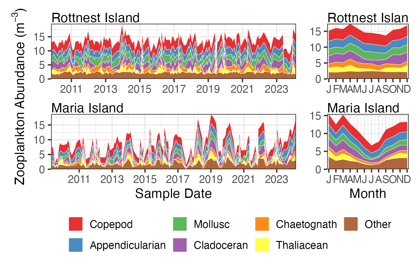
Continuous Plankton Recorder
Have a look at the file and see what is available for plotting, by downloading the file you can inspect the parameters and the bioregions available.
CPRz <- planktonr::pr_get_Indices(Survey = "CPR", Type = "Zooplankton")
unique(CPRz$Parameters)
#> [1] "BiomassIndex_mgm3"             "ZoopAbundance_m3"
#> [3] "CopeAbundance_m3"              "AvgTotalLengthCopepod_mm"
#> [5] "OmnivoreCarnivoreCopepodRatio" "NoCopepodSpecies_Sample"
#> [7] "ShannonCopepodDiversity"       "CopepodEvenness"
#> [9] "PCI"
unique(CPRz$BioRegion)
#> [1] "South-east"            "None"                  "South-west"
#> [4] "Southern Ocean Region" "North-west"            "North"
#> [7] "Temperate East"        "Coral Sea"
Trend Analysis
Here we can compare the long term time series copepod abundance data for the South-east and Temperate-east areas of Australia. Due to way the CPR data is collected this is easier to visualise in a regional context. There is not a noticeable difference in the abundance of copepods in these two regions from the plots but again you can see that the seasonal cycle is more distinct in the South-east.
CPRz <- planktonr::pr_get_Indices(Survey = "CPR", Type = "Zooplankton") %>%
  filter(Parameters == "CopeAbundance_m3") %>%
  filter(BioRegion %in% c("South-east", "Temperate East"))

p1 <- planktonr::pr_plot_Trends(CPRz, Trend = "Raw", method = "lm", trans = "log10")
p2 <- planktonr::pr_plot_Trends(CPRz, Trend = "Month", method = "loess")

p1 + p2 +
  ggplot2::theme(axis.title.y = ggplot2::element_blank()) + # Remove y-title from 2nd column
  patchwork::plot_layout(widths = c(3, 1), guides = "collect")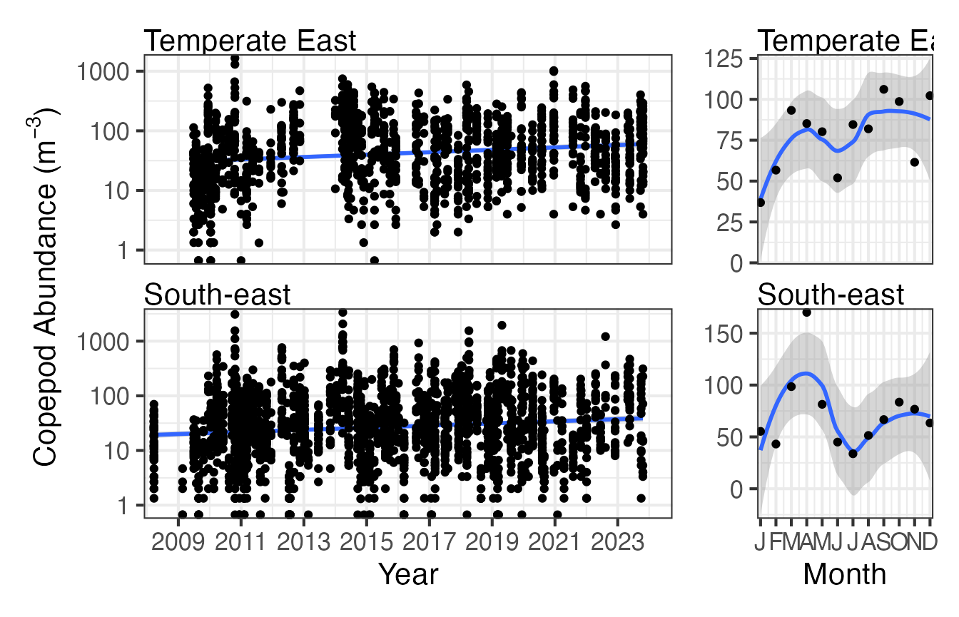
Climatologies
Plotting the same data as climatologies can provide another way to visualise the differences between sampling regions.
p1 <- planktonr::pr_plot_TimeSeries(CPRz, trans = "identity") + theme(legend.position = "none", axis.title.y = element_blank())

p2 <- planktonr::pr_plot_Climatology(CPRz, Trend = "Month", trans = "identity") + theme(legend.position = "none")

p3 <- planktonr::pr_plot_Climatology(CPRz, Trend = "Year", trans = "identity") + theme(legend.position = "bottom", axis.title.y = element_blank())

wrap_plots(p1, p2, p3, ncol = 1)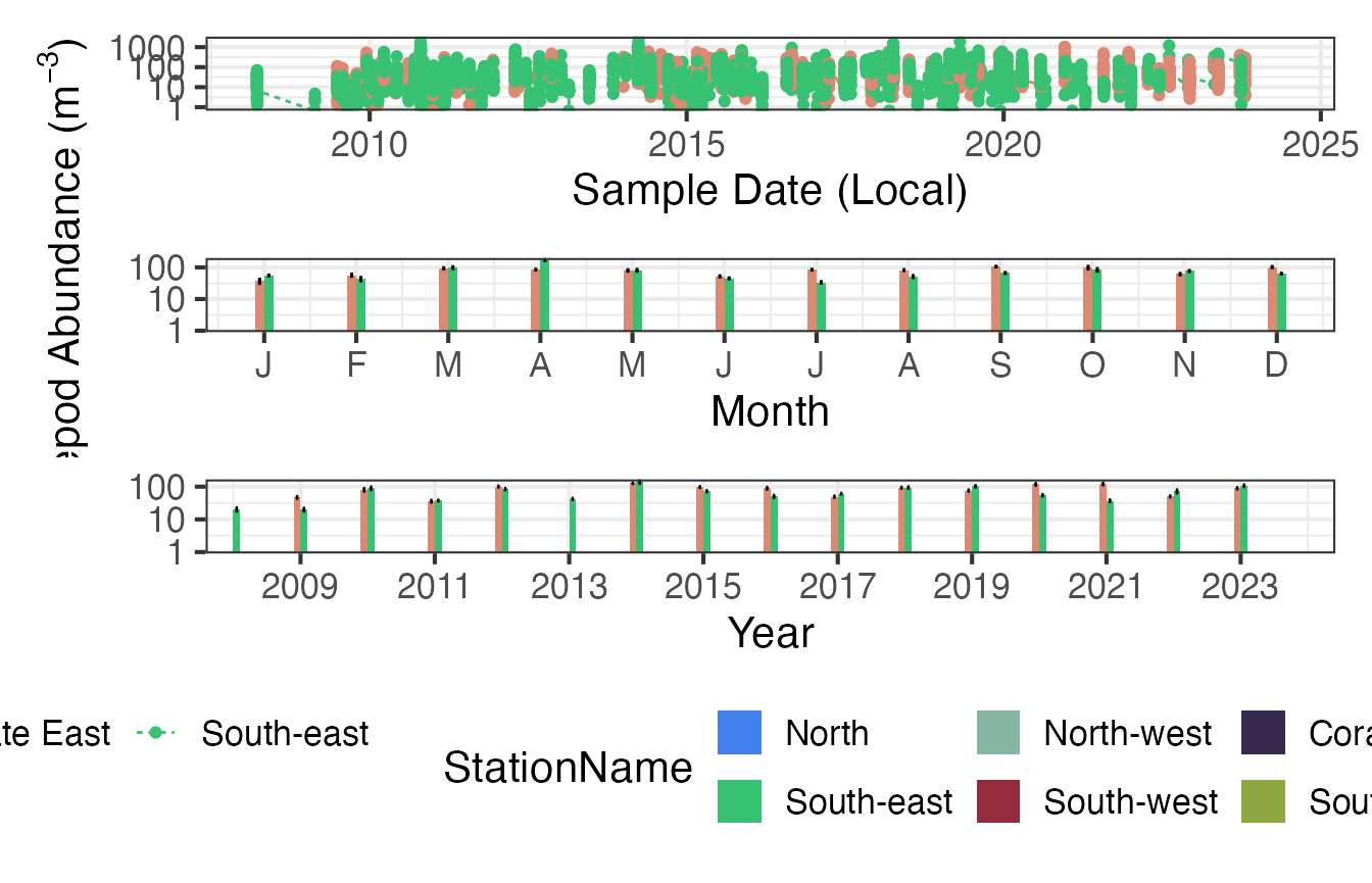
Functional Groups
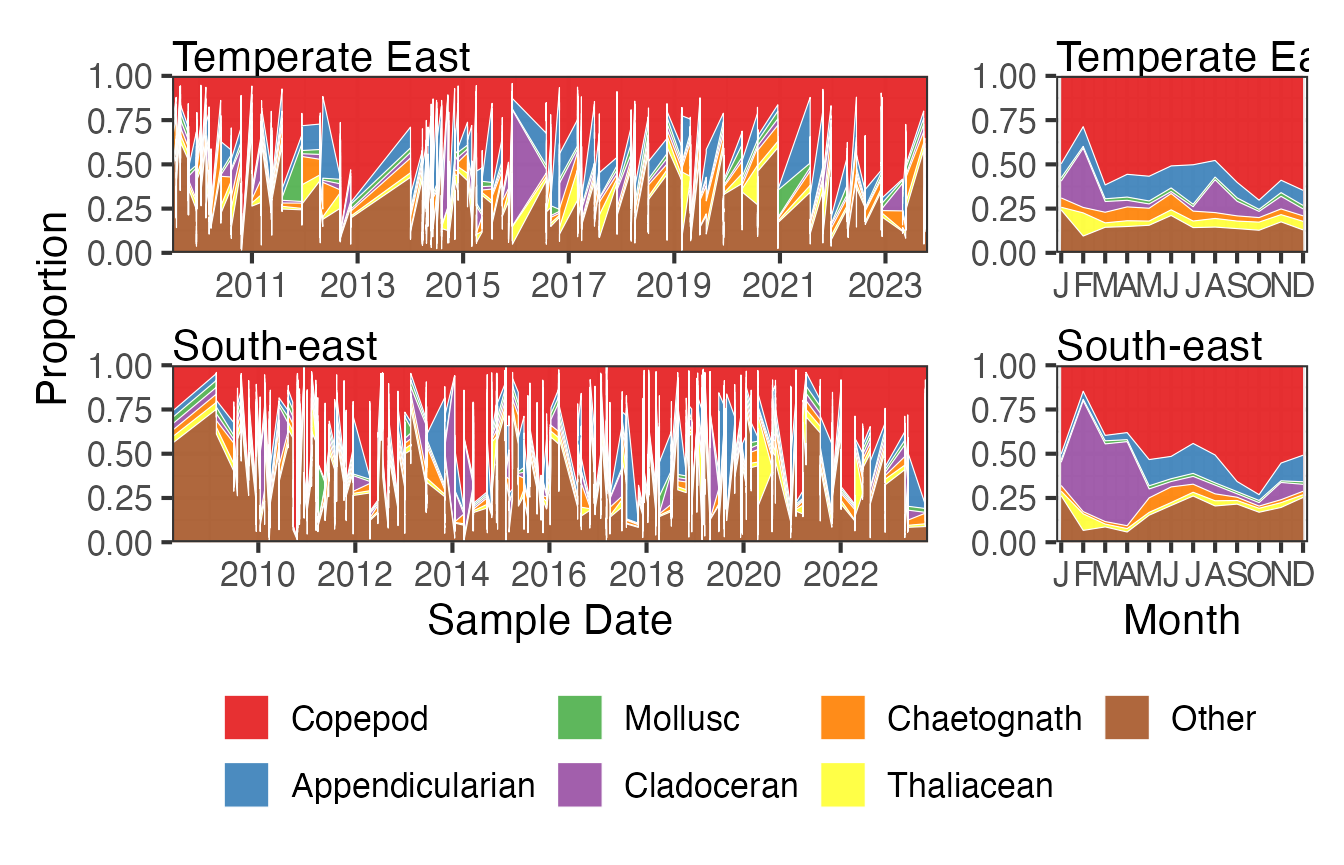
If we look at way the proportion of different functional groups varies over time we can see that copeopds, red, dominate the plankton in both areas, especially towards the end of winter, and that there is a notable bloom period of cladocerans in the South-east over the summer months.
FG <- pr_get_FuncGroups(Survey = "CPR", Type = "Zooplankton") %>%
  filter(BioRegion %in% c("South-east", "Temperate East"))

p1 <- planktonr::pr_plot_tsfg(FG, Scale = "Proportion")
p2 <- planktonr::pr_plot_tsfg(FG, Scale = "Proportion", Trend = "Month") +
  ggplot2::theme(axis.title.y = element_blank())

p1 + p2 +
  patchwork::plot_layout(widths = c(3,1), guides = "collect") &
  theme(legend.position = "bottom")